PARALLEL PROCESSING

Computer Programs and Parallelism:

A computer program consists of a sequence of instructions. Each of these instructions performs some operations on certain data operands. So, computer program can be considered as a sequence of operations on certain data operands. A computer program is said to exhibit parallelism, if these operations (to be performed on data operands by the given set of instructions) can be performed in any order. If the operations could be performed out of order, and multiple processing elements (or ALUs) are available, then it would be possible to perform these operations in parallel (since the order of execution does not matter) at the same time. That is where the world parallelism coins from. The processors which provide multiple ALUs on a single chip (to exploit the program parallelism) are called parallel processors (and the process is known as parallel processing) . There could be different kind of parallelism in a program.

Instruction Level Parallelism
Data Level Parallelism
Thread Level Parallelism

Instruction Level Parallelism:

Consider the following instruction sequence

data1 = data2+data3;
data4 = data2+data5;
data6 = data3;

Changing the order of above instruction does not effect the final result (values of data1, data4 and data6 will remain same). Since the instructions can be executed out of order, we can execute them on three different ALUs (provided that the processor on which you are executing your instructions has multiple ALUs available) in parallel. This is called Instruction Level Parallelism. There are no dependencies in the above instruction. However certain dependencies amongst the instructions can exist. In such a scenario, the instructions depend on each other and can not be executed in parallel (certain dependencies can still be resolved using some techniques). Consider the following sequence of instructions:

data1 = data2+data3;
data2 = data4;
data5 = data2+data1;
Changing the order of above instructions, will change the program results (final values of data1, data2 and data5).

There can be three kind of dependencies:
True Dependencies (or Read after Write)
Anti Dependencies (or Write After Read)
Output Dependencies (or Write after Write)

True Dependencies: (Read after Write)

data1 = data2+data3;
data4 = data1 + data5;

Here the content of data1 are being read after write to data1. This is a true dependency and can not be resolved.

Anti-Dependencies: (Write after Read)

data1 = data2 + data3;
data2 = data4;

Here first instruction depends on the second instruction. If the second instruction is executed before the first, result of first instruction will change (because the value of data2 will be different). Since first instruction here depends on the result of a future instruction, it is said to anti-depend on the future instruction. The anti-dependencies can be resolved using renaming. As shown below, renaming the conflicting variable (data2 in this case), resolves this dependency.

data1 = data2 + data3;
new.data2 = data4;

Output-Dependencies: (Write after Write)

Exists when ordering of instructions will affect the final output value of a variable.

data1 = data2 + data3;
data4 = data1/data7;
data1 = data5+data6;;

Here the re-ordering of instruction-1 and instruction-3 will affect the final value of output variable data4 (instruction-2). Similar to anti-dependencies, the output-dependencies can also be resolved using renaming.
data1.new = data2 + data3;
data4 = data1.new/data7;
data1 = data5+data6;;

Data Level Parallelism

A Data Processing application is said to exhibit Data Level Parallelism, if different data blocks can be executed out of order. One such example is Image Processing applications. In Image processing applications, entire image is divided in to smaller macro-blocks and each macro-block can be processed (generally mathematical transforms) individually. Since each data blocks has to undergo the same operations (same processing), such application can be efficiently run on SIMD (Single Instruction Multiple Data) Architectures, as we will discuss in next section.

Thread level parallelism

Sometimes (data intensive applications), the performance of application is limited by the I/O bandwidth (the rate at which data can flow in and out of the system) rather than the processing power of the system. In such systems, dividing the complete application in to multiple independent (independent at least to some extent) threads, can improve the overall performance. When one task has been blocked due to I/O dependency, the other task can be executed (and first task can take over the CPU resources when it is ready again). In modern days, some companies provide multiple-core CPUs (this is different from a CPU having multiple ALUs). A multi-threaded application can exploit the multi-core design efficiently, since each thread can run on a different core.

Parallel Processing and Pipe-lining

Most modern processor parallelize the operations being performed by its CPU. The Fetch, Decode and execute stages in the CPU are generally pipe-lined, such that when one instruction is being executed, the next instruction will be under decode stage and the next instruction will be under fetch stage.

Cycle          Fetch                    Decode                     Execute 
    T        Instruction-n+2    Instruction-n+1     Instruction-n 
T+1       Instruction-n+3    Instruction-n+2     Instruction-n+1 
T+2       Instruction-n+4    Instruction-n+3     Instruction-n+2 
 ..                  ..                               ..                             ..

The figure above shows a simple three-stage pipeline. However each of these stages can be broken down in to simpler stages which can be further pipe-lined.

Branching

Consider a conditional (If-Else) code as shown below:

 
if (CONDITION one is true)
{
         instruction sequence 1
}
else
{
          instruction sequence 2
} 

Based on whether the CONDITION is true or false, one or other instruction sequence is executed. This is called conditional branching. In most of the cases, CONDITION depends on result of the instruction which have been performed just before this executing this code section.

Branch Prediction

Conditional Branching can greatly impact the performance of a pipe-lined processor. The result of CONDITION check will generally be available only at the end of Execute Stage. Hence which instruction to fetch (instruction sequence 1 or instruction sequence 2) will be known only at the end of execution stage of the instruction which involves conditional check. However, in a pipe-lined processor, the next instruction (next to conditional check in this case) should have been fetched (generally processor fetches the next instruction in the memory) when the current instruction was in decode stage. If result of conditional check required some other instruction sequence to be executed, then processor will need to flush its pipe-line (kill all the instruction in fetch and decode stages) and start fetching instructions from a different location.
Simple processors have a three stage pipeline. However, most modern processor include several pipe-line stages. Each of the Fetch, Decode and Execute operations are further pipe-lined. Therefore frequent pipe-line flush operations (caused by conditional branching) can cause a major performance hit on processor which have multistage pipeline.
Processor architectures use Branch Prediction Technique to improve the processor performance with conditional branches. Branch condition could be dynamic or static. Under static branch prediction use can optionally specify a qualifier in the conditional branch instruction. If this qualifier is specified, then processor will start fetching instructions from the branched location (the location from where code shall be executed in case branch happens) after fetching the current instruction. If no qualifier is specified, then processor will keep fetching the instructions linearly. The Branch Prediction qualifier could be used by the programmers, based on probability of conditional branch. If probability of taking a branch is higher, then BP qualifier shall be specified as part of the instruction. Under Dynamic Branch prediction, a dedicated hardware takes care of the branch prediction. This hardware maintains a statistics of previous branches and based on this data it dynamically adapts the branching logic.

A Pipeline Example

Let us consider the example of Blackfin Processor (BF-533). Blackfin Processor has a ten-stage pipeline. There are three Instruction Fetch Stages, Four instruction Decode Stages (which include two stages of data fetch) and three execute stages (which includes result write-back) stage.

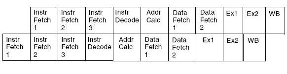
As we discussed in the previous section, in case of a branch, the program sequence will need to flush the entire pipe-line. The result of the conditional instruction becomes available at the end the second execution stage. Hence there will a penalty of eight clock cycles (eight stages in the pipe-line will require a flush). The Branch Address (in case of a conditional branch) becomes available after the end of "Addr Calc" (Address Calculation) stage in the pipe-line. Hence if branch-prediction is enabled, still the program sequence will need to flush 4 stages in pipeline (because branch address is not available until then).

Program Sequencer

The Program Sequencer in a Processor is responsible for fetching instructions from the memory. Normally, the program sequencer executes a linear code. However, there are certain conditions when program sequencer can jump to a non-linear instruction address. One such condition is a function call (this is also known as sub-routine call). Another condition we discussed in one of the previous section, was a conditional branch. Function (or subroutine) call is generally implemented using a "CALL" instruction (CALL instruction also contains the address of function being called with as part of the instruction) in assembly language. Branching (conditional or un-conditional) is generally implemented using a "JUMP" instruction in assembly language. I have mentioned about JUMP and CALL because these instructions are available in instruction sets of many processors, however similar instruction might have a different name on a specific processor (but the this discussion will still be applicable irrespective of the instruction name). Both JUMP and CALL instruction are similar in the sense that they break the linear code flow in an application and make the program sequencer to fetch an instruction from a new (non-linear) location. However these is a significant difference between JUMP and CALL. When a processor executes a CALL instruction, it stores the current linear address (Address of the instruction next to the CALL instruction) in one of the processor registers, this address is called Return Address. At a later stage (when the called function has finished its work), and RTS instruction (Return from Subroutine) will bring the program flow back to the Return Address. Therefore, a function (or subroutine) should contain RTS as its last instruction. However, there is not Return Address associated with a JUMP Instruction.

User Comments